Showing posts with label algorithms. Show all posts

Wednesday, June 26, 2013

More on Genetic Algorithms: How They Can Be Used in Engineering Optimization Problems and Mate Selection Techniques

In a previous post, I gave a brief introduction to Genetic Algorithms (GAs), how they work, and how they can be used in antenna optimization problems. Today, I want to give a more detailed explanation of how GAs select mates for reproduction. I show a block diagram of a simple genetic algorithm (SGA) with elitism in Figure 1 below.

Figure 1: Block diagram of a simple genetic algorithm (SGA) applied to an anti-jamming antenna array optimization problem (Copyright Jonathan Becker)
The SGA shown above is setup to solve an anti-jamming beamforming array optimization problem, as the fitness function is the array's signal to interference and noise ratio (SINR). However, GAs can be used for a wide variety of (difficult) engineering optimization problems provided that the fitness function is defined according to the design requirements associated with those problems. Remember that fitness functions are maximized in GAs, as the goal is to find the fittest (i.e. best) solution or solutions. In order for the fitness function to be useable, it must have the following characteristics:

  1. All possible fitness function values must be greater than or equal to zero.
  2. The fitness function must not be binary (i.e., having only two values such as 0s or 1s).
  3. The fitness function must be finite. In other words, it cannot possess any singularities.
The third condition is obvious, as no computer can evaluate infinite valued functions. I will explain the reasons for the first two conditions after I discuss the common types of fitness proportional mate selection methods used with GAs:
  • Random (i.e., biased roulette wheel) select
  • Stochastic remander select
  • Tournament select
In the random fitness proportional mate selection method, a string i (where 1 < i < M) in generation n (where 0 < n < N) is selected with probability according to


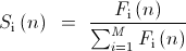
This equation is essentially a probability because it equals string i's fitness function value divided by the sum of every string's fitness value (i.e., the population's total fitness). Here's the reason why the fitness function values must be non-negative: It doesn't make sense to calculate probabilities with negative numbers. Of course, the fitness functions must not be infinite, or selection probabilities would be zero for all strings, and no strings would be selected as mates. The general idea is that strings with higher fitness will be chosen more often than strings with low fitness. For this reason, the fitness function must not be binary because the algorithm would be either hit or miss. Unless the GA was lucky and found the solution out of pure, blind luck, it would go nowhere and not optimize the problem's solution.

A major issue with random select, however, is that it has high variance meaning that strings with low fitness will sometimes be selected for mating. You can think of random select as a biased roulette wheel where the width of each slot has an area proportional to each string's fitness. Suppose that the 15th slot out of 100 spokes has the largest area. Your best option would be to place your bets on slot 15. Although the ball will land on slot 15 on average out of N spins, it will occasionally land on other slots, and you'll lose your money whenever that happens.

Now, stochastic remainder select reduces mate selection variance by calculating the expected count of any given string i and separating that count into integer and remainder portions according to


Stochastic remainder select deterministically selects that string Int times and selects it one more time with probability (0 to 1) equal to R. Note that FAvg is the average fitness in any given generation. Because most of the selected strings are chosen deterministically, and the last string is chosen with probability R, stochastic remainder select has a much lower variance than random select. The random (i.e. stochastic) part of stochastic remainder select is equivalent to flipping a biased coin only once. 

In addition, tournament selection, as I understand it, randomly selects a small group of strings. The strings compete against each other (as in a tournament), and the string with the highest fitness out of the group is selected for mating. The process is repeated with another group of strings to select the second mate. The strings that are selected are removed from the tournament, and the process is repeated until anywhere from half to three quarters of the population is selected. To preserve good solutions, half of the population is typically selected for mating while the other half is typically copied from the parent generation without crossovers and mutations. The copied (i.e., elite) strings are the best strings from the parent population while the strings chosen for crossover and mating are the worst half. I don't use tournament selection because I believe that it forces a lot of genetic material to be lost. I prefer to use stochastic remainder select because I found that it works both in simulations and in situ with hardware, and the majority of the parent population's genetic material is used to create the children population.

There are other other types of mate selection methods, but the three I described are most commonly used with random select being the first method developed in GA computer science theory. I've also explained what properties the fitness function must have in order for it to be used in a GA. Because of its ability to search multiple sections of the solution search space in parallel, the GA can optimize many multi-objective engineering problems including rocket nozzle design (i.e., maximizing thrust while minimizing nozzle weight), metallic bridge design (i.e., maximizing load handling while simultaneously minimizing weight), and so forth. The GA can create viable and unique solutions that few humans could design by hand alone. 


Best,

Jonathan Becker
ECE PhD Candidate
Carnegie Mellon University

Monday, June 24, 2013

An Introduction to Particle Swarm Optimization (PSO) with Applications to Antenna Optimization Problems

I'm in the early stages of research Particle Swarm Optimization (PSO) and applying it to evolving my anti-jamming beamforming antenna arrays. By early, I mean that I've been reading books and articles on PSO. I have not yet written my own PSO codes, nor have I tested any PSO code on my antenna array. With my next antenna array, I hope to do experiments with my own PSO code and compare PSO performance to that of the genetic algorithm (GA) with an interim goal of publishing a conference paper and an end goal of publishing my thesis. In this post, I will give an introductory explanation of how PSO works, and how it applies to antenna optimization.

PSO is a stochastic optimization algorithm developed by computer scientists to solve difficult problems.  (By difficult, computer scientists mean that the problem cannot be easily solved by simpler optimization algorithms like Newton's Method, simplex methods, gradient descent, and/or Least Mean Squares.) Like the GA, the PSO is a population based search algorithm that integrates randomness in a guided search of the parameter / solution space. However, the PSO is modeled after social behaviors instead of "survival of the fittest" mate selection and genetic chromosomal crossovers and mutations.

Think of a swarm of animals (like bees, birds, fish, or even people) searching for a food source. In the beginning of their search, the swarm will be randomly spread out with various positions and velocities as shown below in Figure 1. PSO is a minimization algorithm meaning that it searches for solutions that minimize an objective function. In this example, the blue star represents a minimum that the PSO needs to find. Each particle records its own minimum (i.e., best) solution as well as the globally best solution. One should note that the globally best solution is not necessarily the optimization function's global minimum: It is simple the best solution found by the swarm so far by the current iteration. In other words, the particles communication with each other, as they tell each other where they're located, and the swarm will propagate itself toward the particle closest to the objective function's minimizer (i.e., food source)

Figure 1: Conceptual diagram of PSO in action with a single global minimum (Copyright Jonathan Becker)
As noted, each particle is characterized by both its position in the search space and its current velocity. Technically, a particle's velocity is just a vectorial change in position. However, computer scientists call this quantity a velocity because the time unit is always one iteration. In its original form, Parsopoulos et. al. [1] noted that the PSO had no means of stopping: The swarm would simply oscillate around the minimizer. Paropoulos et. al. later added a linearly decreasing inertia weight to slow the particles' velocities. They found that this caused the swarm to settle on the minimizer as expected.

Of course, PSO would be better suited at multimodal optimization problems that have local minima as well as a global minimum. I give example of how the PSO might behave in minimizing a problem that has two non-equal minima in Figure 2. I've labeled the two minima A and B. At iteration N, the swarm is divided between solutions A and B. How the swarm behaved depends on whether A is the global minimum or if B is the global minimum. In either case, the swarm will eventually migrate towards the global minimum, in theory any way.

Figure 2: PSO example with two non-equal minima (Copyright Jonathan Becker)
I would like to point out another differing quality between PSO and genetic algorithms. (GAs are used in maximization optimization problems, but a minimization optimization problem can be easily converted into a maximum optimization problem.) Suppose that B is the global minimum. You may notice that there are particles at iteration N that are not near B nor A. The GA would simply kill these solutions off, as they would have low fitness function values. However, PSO does not remove particles from the swarm, and particles communicate with each other. The particles not near a minima would move towards the direction of the best solution found so far. Of course, the information might get diluted, as Clerc noted that a given particle might find a better solution at the next iteration and move in a different direction [2].

In the reading stage of my research, I am finding that there are multiple variants of PSO each of which attempts to solve deficiencies that earlier variants possessed. At this stage of my research, I have not decided which PSO variant I will use in solving the anti-jamming beamforming problem, or if I will attempt to create a new variant. What I do know is that I'll want my PSO code to tackle mobile signals (i.e., moving signals of interest and/or moving jammers), so I won't want to use an inertial dampening term that completely diminishes the swarm's searching abilities.

Other researchers have used PSO to optimize antenna designs as well as antenna arrays for focusing electromagnetic energy in the direction of a signal of interest [3 - 5]. The procedure for optimizing antennas with a PSO is similar to the procedure used by the GA to optimize antennas. Except, the objective function is defined with minimization (not maximization) in mind. I list the steps below for optimizing an antenna design using a PSO:

  1. Define the type of antenna that will be optimized: Yagi, log-periodic, helix, custom design, etc.
  2. Define the problem parameters that need to be minimized: antenna gain, impedance matching, antenna physical size, etc.
  3. Define the objective function to be minimized with the problem parameters in mind. For techniques on multiobjective optimization, refer to the text written by Deb [6].
  4. Generate a randomly defined population. Some PSO variants generate a uniformly distributed population, others apply another optimization algorithm (such as simplex) to prime the population before starting the PSO. (Parsopoulos noted that this gives better results overall [1].)
  5. Run the PSO for a predefined number of iterations.
  6. Stop the PSO when a design that meets the design specifications is found or when the maximum number of iterations is run, whichever comes first.
  7. If the final best solution does not meet the design specifications, consider another antenna design by going back to step 1 or relax the problem parameters / specifications in step 2 and rerun the PSO from there.
  8. If the best solution meets the design specifications, fabricate the antenna and test it.
The steps above assume that the antenna designs will be simulated with a computer and then built to be tested for verification. In antenna array optimization in-situ with hardware (i.e., my research), the PSO would be run on a machine (whether computer, FPGA, etc.) while simultaneously optimizing the antenna array hardware. Typically phase shifters and step attenuators settings are set by the optimization algorithm not the antennas themselves. It is possible to adapt a reconfigurable antenna array by adjusting the shapes the antennas or of the array itself, but this is harder (and possibly slower) than adjusting only phase shifters and step attenuators because it involved mechanical mechanisms

In a nutshell, that is how particle swarm optimization works and how one would apply it to antenna optimization problems. In addition, I've listed my reference below for anyone who wants to learn more about PSO and its application towards antenna / antenna array optimization below. There are certainly other references out there, but these would be a good start for learning about PSO and its applications towards antenna optimization.


Best,

Jonathan Becker
ECE PhD Candidate


References:
[1] K. E. Parsopoulos and M. N. Vrahatis, Particle Swarm Optimization and Intelligence: Advances and Applications, Hershey: Information Science Reference, Hershey, PA, 2010.

[2] M. Clerc, Particle Swarm Optimization, ISTE USA, Newport Beach, CA, 2006.


[3] M. Benedetti, G. Oliveri, and A. Massa, "Validation of a smart antenna prototype: model and experiments." In 2009 European Radar Conference, EuRAD 2009. pp. 172–175, September 30 2009 - October 2, 2009.

[4] H. Huang, A. Hoorfar, and S. Lakhani, "A comparitive study of evolutionary programming, genetic algorithms, and particle swarm optimization in antenna design." In 2007 IEEE Antennas and Propagation Society International Symposium, pp. 1609–1612, June 2007.

[5] M. Ohira, A. Miura, M. Taromaru, and M. Ueba, "Efficient gain optimization techniques for azimuth beam/null steering of inverted-F multiport parasitic array radiator (mupar) antenna." IEEE Transactions on Antennas and Propagation, Vol. 60, Num 3, pp. 1352–1361, 2012.

[6] K. Deb, Multi-Objective Optimization Using Evolutionary Algorithms, Wiley, 2009.


Friday, June 21, 2013

Benefits of Earning an Engineering PhD or Why Bother With all That Hard Work?

As you know, one must put a lot of hard work and dedication into earning a PhD degree especially in an engineering subject. It is only natural to ask: Why even bother? What do I get out of earning such a degree when I could get a job in industry with only a Bachelor of Science? Today, I will explain the benefits of why one would earn a PhD degree.

Before I explain the benefits, there are several reasons why you would pursue a PhD degree:
  • You love doing groundbreaking research and publishing papers on your research
  • You love getting in front of people and presenting your work and ideas
  • You love doing hard work and have a passion for what you do
  • Your career has hit a slump and you are not interested in management
  • You really love academia and the idea of sitting in a cubicle 8+ hours a day frightens you
  • Your career goal is to become a professor, so a PhD is required
  • You want to earn more money compared to other entry level jobs in your industry
  • And so forth...
The main benefit of earning a PhD degree is that you become an expert in at least one field. I say "at least" because the old adage of a PhD'er being pigeon holed into a vary narrow area of expertise with no knowledge whatsoever of other subjects is no longer true. In the Electrical and Computer Engineering Department at CMU, PhD students are required to take courses in at least three different areas. My breadth areas, for example, are electromagnetics (i.e., antennas), probability and random processes, and optimization. Because my research is applied, I have to know multiple areas in order to get good, repeatable results. I've also become an expert in Matlab particularly in controlling lab instruments and such because Matlab is so versatile. As far as industry recruiters are concerned, this makes me a valuable asset because I have accumulated a wide span of engineering experiences.

In addition, you have many opportunities to build your professional network. You start with your PhD advisor, as he/she has contacts in both industry and academia. Don't forget about attending conferences, as you can meet experts in your field who you can interact with during your presentation question and answer sessions as well as during the conference itself. Of course, your classmates become part of your network simply because you will work with them, discuss your research, have fun at department events, and become very good friends -- all through the lifespan of your PhD.

Furthermore, you solidify your knowledge and ad to your engineering field by publishing conference and transactions papers. It is a good experience to write papers, as you get practice in clearly telling the stories of your research. This also helps you remember what you learned in your graduate courses and during your research because writing your thoughts down set them into your memory. There is another benefit, of course, for publishing papers: You can get your name out there by publishing conference and transactions papers. For example, if you go to Google Scholar and type ("Jonathan Becker" and "Carnegie Mellon") as between the parentheses, the top three listing are papers I published with my advisor and his business partner. Think about it. Potential employers can Google you and download your work, and they can read what you wrote. This will help them understand what you do before you have interviews with them. It also makes you look really good in their eyes assuming that you did good research and told your "story" clearly.


Best,

Jonathan Becker
ECE PhD Candidate
Carnegie Mellon University

Hamerschlag and Roberts Engineering Hall (Copyright Jonathan Becker)

Thursday, June 20, 2013

What it Means to Earn an Engineering PhD Degree

In my experience, many people outside of academia do not understand what it means to earn an engineering PhD degree. I believe this is because many people have not gone through the process of earning a PhD degree. There is nothing wrong with this because a PhD degree takes four to five (or more) years of commitment to hard work, long hours, a lot of stress, and often low pay. In this post, with an accompanying vlog, I explain what it means to earn the PhD degree.


As I pointed out in the video, an engineering PhD degree primarily focuses on graduate level engineering research. Unlike a Bachelor degree, the PhD degree is therefore less loosely defined because each PhD student do different kinds of research. There are some well defined requirements to the PhD degree, such as:
  • Graduate level courses related to your research
  • Required Teaching Assistant (TA) positions
  • Qualifier exams to show that you can do quality research (MUST PASS OR ELSE!)
  • Thesis proposal or prospectus
  • Thesis on the PhD student's research
  • Dissertation (i.e. defend the thesis during a long presentation)
There is one question that PhD students really don't like to be asked, but people ask us anyway: When will you finish your PhD? Please understand that it's not that we don't like people asking us questions. It's that we really don't know the answer ourselves, and it becomes our nature to be experts in what we do. It just throws us off guard when someone asks a question that we don't know how to answer.

The reason that PhD students don't know when exactly they'll graduate is that the decision is not based on a clearly defined set of requirements. PhD students graduate when they've successfully defended their thesis in dissertations. However, it's really up to the PhD advisor and the thesis committee members to decide when PhD students are ready to defend their thesis. Because each thesis committee is different, it's impossible to predict how much effort a PhD student will need to put into writing a thesis before the committee feels the thesis is ready to be defended. The PhD student regularly communicates with his/her committee members and gives them updates on his/her research. Now, the committee members can like the research that the PhD student has done so for, or they can ask the student to redo the research or do more research.

In my case, I hope to be done in a year because that's how long my PhD advisor believes it will take me to finish my research, write my thesis, prepare my dissertation, and defend my thesis in the dissertation. This could all change as I write my thesis. I hope not because I really want to finish by this time next year.


Sincerely,

Jonathan Becker
ECE PhD Candidate
Carnegie Mellon University


Hamerschlag Hall Smoke Stack

Monday, June 17, 2013

Anti-Jamming Beamforming Arrays Optimized with Genetic Algorithms: A Recap

Today, I've decided to give a recap on the research that I do since I've written on several subjects during the last week. I'm researching different stochastic algorithms for optimizing anti-jamming beamforming arrays. To date, I've researched the effectiveness of genetic algorithms at doing this task. I've included a YouTube video that I created a while back that explains how the array works.


The above array consists of four antennas, phase shifters, step attenuators, a 4-way RF power combiner, and digital controllers. The array operates by adjusting phase and attenuation on the three outer antennas. The end goal is to focus RF energy on the signal of interest while simultaneously minimizing (i.e., nulling) RF energy in jammer directions. I used a genetic algorithm (GA) to optimize my anti-jamming antenna array. The genetic algorithm (GA) controls the phase shifter and step attenuator settings based on survival of the fittest mate selection, bit-wise chromosomal crossover, and bit-wise chromosomal mutations. The figure below shows a flowchart of the GA. In my research application, the GA uses signal to interference and noise ratio (SINR) as its fitness function.

Figure 1: Flowchart showing how the GA operates to maximize SINR (Copyright Jonathan Becker)
In the figure above, the signal of interest that you want to receive is the signal portion of SINR, and the jammers are the Interference portion. An initial population of binary settings are created, decoded into hardware settings, and evaluated to create the SINR fitness functions. Crossovers and mutations are applied with probabilities p(cross) and p(mutation). I assume that noise is additive white Gaussian noise (SINR) and is dependent on the system bandwidth and ambient temperature. The new solutions (i.e., children) are decoded into hardware settings and reevaluated. The whole process is repeated until a solution with an acceptable fitness function is found or the algorithm reaches a maximum number of iterations (i.e., generations). If you wish to learn more about how the GA works, please read my previous post on genetic algorithms.

In future research, I will compare other stochastic algorithms such as Particle Swarm Optimization (PSO) with the GA. I will likely build a new antenna array build with surface mount components on printed circuit boards (PCBs). This array will have eight antennas to increase the maximum number of jammers it can thwart. I'm also considering using wideband antennas, so the array can operate on multiple bands. Come back and visit my blog, as I plan on writing on these and other technical subjects, and I will give other tips on surviving graduate school.


Your truly,

Jonathan Becker
ECE PhD Candidate
Carnegie Mellon University

Tuesday, June 11, 2013

Simulated Annealing: Modeling Metallurgical Annealing to Solve Engineering Optimization Problems

Although my research in antenna arrays primarily focuses on genetic algorithms, I have studied other stochastic algorithms during the course of my PhD. One such algorithm is known as simulated annealing. Like genetic algorithms, SA is based on a process that occurs in nature. However, simulated annealing is not population based, and it is based on a physical process instead of a biological process.

The concept behind simulated annealing is simple. It is analogous to a blacksmith tempering steel to make a sword. The blacksmith heats the metal to a very high temperature and lets the sword cool slowly as indicated in Figure 1. This process makes the sword stronger than the untreated steel. However, if the blacksmith suddenly tosses the hot sword into a cold water bath, the steel would become brittle. This is certainly not good, as the sword could shatter when it strikes another sword or hard surface.

Figure 1: Sword Annealing Analogy to Explain Simulated Annealing (Copyright Jonathan Becker)

Of course, annealing works at the atomic level as shown in Figure 1. When the steel is heated to a very high temperature, the atoms move very fast in random directions. As the steel cools, the atoms begin to slow down. If the steel is cooled at just the right rate, the atoms will settle into a perfect crystalline lattice. However, if you cool the metal too fast, the crystalline lattice will have imperfections in it, and the steel will be of lower quality. You can cool the object too slowly and still get good results, but you'll wait too long to see the results.

From the example above, you can see the main steps behind simulated annealing:
  1. Start with an "object" that has M "atom" positions in random positions.  This is iteration n = 0, and the solution is named S(n=0).
  2. Heat the "object" to a very high temperature, say 1000 Kelvins.
  3. Cool it slowly according to a predefined temperature schedule until it reaches a low temperature, say 0 Kelvins, where the "atoms" are frozen in their current state. The algorithm runs for a total of (N + 1) iterations, i.e. 0 < n <= N.
    •  At each iteration n, generate a new solution S(n+1) with a probability Ps(n+1) defined by the temperature schedule. If a new solution is not generated, S(n+1) = S(n).
    • If S(n+1) is better than S(n), keep solution S(n+1). Otherwise, keep S(n).
  4. Compare the end result with the optimization requirements. If the result does not meet the acceptance criteria, discard it and go back to Step 1.
The trickiest part of getting a simulated annealing program to produce good results is in choosing the right temperature schedule. Typically, one would choose a sigmoid temperature schedule (shaped like the letter "S") like the one shown in Figure 2.  Of course, there are other types of sigmoid functions available (such as an arctangent function offset by 90 degrees). One chooses the parameters of the sigmoid function through multiple simulations.

Figure 2: Example Sigmoid Temperature Schedule.  Cooling rate (tau) and offset "a" need to be chosen carefully.
A sigmoid temperature schedule starts at a high temperature such that Ps(0) = 1 (or close to 1), and it decays slowly at first, so the algorithm can effectively search the parameter space. As the number of iterations "n" increase, the schedule decays faster allowing the algorithm to settle into a crystalline lattice. As the algorithm nears completion, the temperature schedule settles out such that Ps(N) = 0. This finishes the cooling cycle and ensures that the best solution is preserved.  You can note that the algorithm is purely random at the beginning of its search and becomes more deterministic as the number of iterations approaches N. The shift from complete (or nearly complete) randomness near the beginning of the with a gradual shift to complete determinism at of the run ensures that the best solution the algorithm found is preserved.

To date, my use of simulated annealing in my PhD research has been limited to antenna placement simulations. Because the test equipment used in CMU's wireless lab was old and slow, I found it impractical to optimize my beamforming array hardware in situ with a simulated annealing algorithm. However, I hope to build a new array this Fall semester that can be attached to a Universal Software Radio Protocol (USRP) device. This would allow me to optimize the new array in a non-ideal environment (i.e. lab space outside antenna chamber) with faster test times. Hence, it would be more practical for me to evaluate simulated annealing at that time.


Best,

Jonathan Becker
ECE PhD Candidate
Carnegie Mellon University

P.S. For anyone interested in learning more about simulated annealing, I highly suggest reading Laarhoven's and Aarts' text Simulated Annealing: Theory and Applications. More info can be found on Google Books.

Monday, June 10, 2013

An Introduction to Genetic Algorithms with Applications to Antenna Arrays

Previously, I discussed testing antenna arrays inside an anechoic chamber, and I explained the setup for testing an antenna array inside an anechoic chamber (see Figure 1 below).  I briefly mentioned that I've researched the use of genetic algorithms (GAs) in evolving antenna arrays to focus electromagnetic (EM) / radio frequency (RF) energy on a signal of interest (SOI) while simultaneously minimizing EM/RF energy in jammer directions. In this article, I will explain how GAs work and how I've used them in my research.

Figure 1: Test setup diagram of antenna array in anechoic chamber (Copyright Jonathan Becker)
The GA was originally developed by John Holland [1] in the 1970s with an update to his classic text in 1992, and was developed further by David Goldberg [2] and Kenneth De Jong [3]. The most basic of GAs is known as the Simple Genetic Algorithm (SGA), and it has three evolutionary operators: "survival of the fittest" mate selection, crossover, and mutation. It is through these three operators that the SGA searches for optimal solutions to a given problem. Typically, a GA is used to find a maximal (i.e., best) solution although it can be modified to solve minimization problems a modification to the fitness function.

Before I can explain the SGA's three evolutionary operators in details, I need to explain a few concepts relevant to GAs in general. First, there is the concept of a fitness function. The fitness function measures how good a solution is in solving a maximization problem. In my research, I use GAs to maximize the Signal to Interference and Noise Ratio (SINR) because maximizing SINR ensures that the GA has thwarted jammers while focusing energy on a SOI. Of course, not all optimization problems involving maximizing some quantity. For example, suppose that you want to minimize the weight of a mechanical part to be installed inside an unmanned aerial vehicle. To apply a GA to this problem, you would first define the objective function to be minimized and invert it while adding a small number in the denominator (to prevent an infinite result). This converts a minimization problem to a maximization problem.

Second, GAs operate on strings equivalent to chromosomes in biology. Typically, the strings are binary (i.e. 1s and 0s) valued although they can be real valued depending on the application. SGAs operate on singly stranded haploid binary strings, and more complicated GAs can operated on doubly stranded diploid strings [4,5]. Third, GAs operate on a population of strings. This allows the GA to search multiple sections of the solution space in parallel -- a property Goldberg called "implicit parallelism" [2]. I show flowchart of the SGA used to maximize SINR in solving the anti-jamming beamforming problem below in Figure 2.

Figure 2: Flowchart of Simple Genetic Algorithm (Copyright Jonathan Becker)
I created the flowchart to explain the concepts of mate selection, crossover, and mutation. The GA chooses pairs of strings based on their fitness using "survival of the fittest." This means that strings with higher fitness are more likely to be chosen than strings with low fitness. In fact, lowly fit strings are likely to die out in the generation that they occur. After the GA selects mating pairs, it performs chromosomal crossover. This is much like crossover in biology where two chromosomes are split and the tail ends are swapped. The idea behind crossover is to create better solutions (i.e., children) by sharing the good properties of their parents (i.e. the mates). Of course, mate selection and crossover is not perfect, and information can be lost in the process. Some of this information might be necessary in solving the given problem at hand. This is where mutation comes into play, as randomly mutating bits (with a small probability, less than 2%) allows information that was lost to be reintroduced into the population. Mutation is a secondary operator in GAs.

I will close this post with an answer to a common criticism of GAs: If the initial population is chosen at random, that means GAs are random search algorithms. (Random search is not an effective algorithm in solving engineering problems.) This is a misconception of how GAs operate. It is true that the initial populations are chosen at random, and crossover points and mutations are chosen with probabilities Pc and Pm. However, the fitness function guides the GA in its search of the solution space to find maximal solution(s). The fitness function is well defined and allows the GA to efficiently solve a wide variety of engineering problems.

I have listed my references below, and you are welcome to read them if you want to learn more about genetic algorithms.


Best,

Jonathan Becker
ECE PhD Candidate
Carnegie Mellon University


References:
  1. J. H. Holland. Adaptation in natural and artificial systems: an introductory analysis with applications to biology, control, and artificial intelligence. Bradford Books. MIT Press, 1992.
  2. D. E. Goldberg. Genetic Algorithms in Search, Optimization, and Machine Learning. Adison-Wesley, Reading, MA, 1989.
  3. K. De Jong. An Analysis of the Behavior of a Class of Genetic Adaptive Systems. PhD Thesis. 1975.
  4. D. S. Weile and E. Michielssen. "The control of adaptive antenna arrays with genetic algorithms using dominance and diploidy." IEEE Trans. Antennas and Propagation, 49(10):1424–1433, October 2001.
  5. J. Becker, J. Lohn, and D. Linden. "Evaluation of genetic algorithms in mitigating wireless interference in situ at 2.4 GHz." In WiOpt 2013 Indoor and Outdoor Small Cells Workshop, pages 1–8, May 2013.